Interpret Results
Use this guide to understand what the solver produced and evaluate whether the result meets your design requirements. Solver results require interpretation -- the raw material layout is a starting point for engineering, not a finished design.
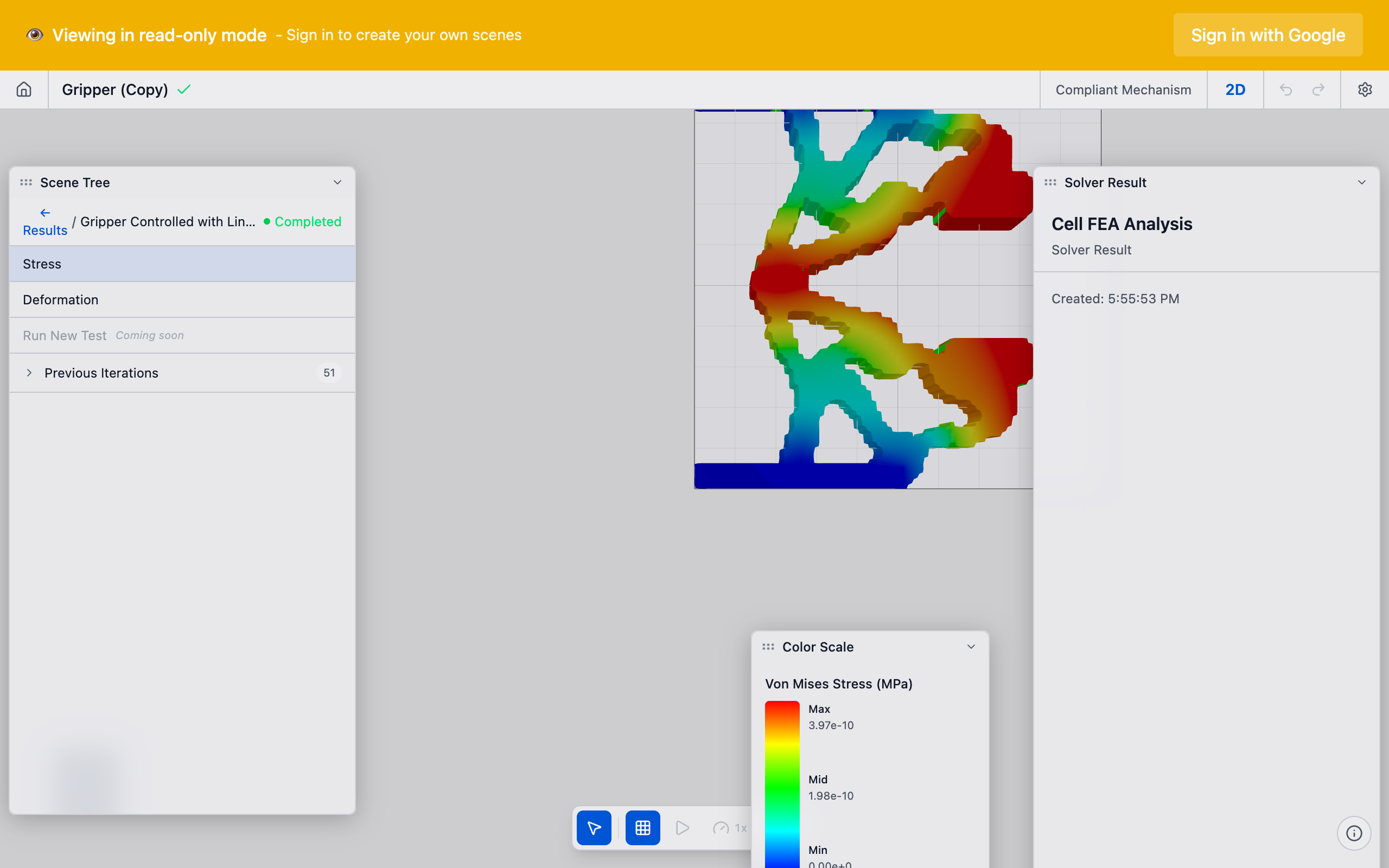
The material layout
The solver output is a material layout: each cell in the mesh has a density value between 0 (void) and 1 (solid). The viewport renders this as a color map:
- Density near 1.0 (dark/opaque): Solid material. The solver determined this region is structurally necessary.
- Density near 0.0 (light/transparent): Void. The solver removed material here.
- Intermediate densities (gray): The solver has not fully committed this region to solid or void. Some gray is normal, especially at boundaries between solid and void regions.
Key metrics to check
Compliance
Compliance is the inverse of stiffness -- lower compliance means a stiffer structure. For compliant mechanisms, the solver manages a trade-off between the compliance of the mechanism (it should be flexible enough to deform) and the mutual compliance (the input-output coupling).
In the solver run summary:
- Final compliance should be finite and positive. A value of 0 or infinity indicates a degenerate result.
- Compliance should decrease over iterations and stabilize. An erratic compliance curve suggests convergence issues.
Volume fraction
The achieved volume fraction should match your target within the convergence tolerance. If you set 0.30 and the result shows 0.32, the solver is within tolerance. If it shows 0.50, something is wrong with the constraint enforcement.
Convergence
A converged run shows the compliance curve flattening in the last 10--20 iterations. If compliance is still changing significantly at the final iteration, the result may not be fully optimized. Options:
- Increase the iteration count
- Decrease the convergence tolerance
- See Solver Not Converging
Evaluating topology quality
Good topology signs
- Clear solid/void separation: Most elements are near 0 or 1, with minimal gray.
- Connected load paths: Continuous structural members connect input preserves to the output through the fixed supports.
- Thin flexural hinges: For compliant mechanisms, you should see thin members that act as living hinges, connecting stiffer regions.
- Preserved regions intact: Bolt pads and other preserves appear as fully solid regions in the material layout.
Warning signs
| Symptom | Likely cause | Fix |
|---|---|---|
| Checkerboard pattern | Mesh too coarse, filter radius too small | Increase filter radius or decrease element size |
| Disconnected islands | Volume fraction too low, preserve placement issue | Increase volume fraction, check preserve positions |
| All gray (no clear topology) | Solver did not converge, too few iterations | Increase iterations, check boundary conditions |
| Solid block with tiny holes | Volume fraction too high | Decrease volume fraction to 0.20--0.30 |
| Topology ignores output | Missing pair, output not linked to input | Check preserve pairs in the sidebar |
See Unexpected Results for detailed troubleshooting.
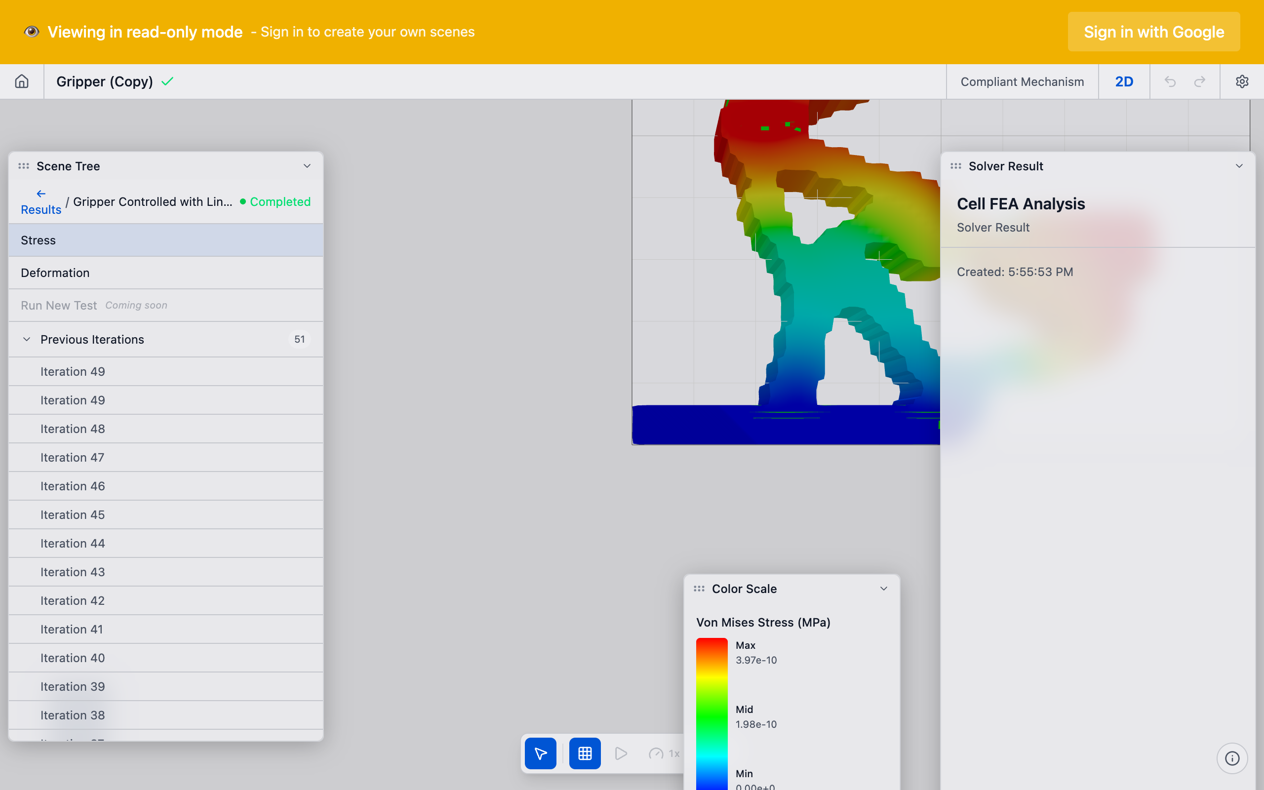
Displacement animation
If available, use the displacement animation feature to visualize how the mechanism deforms under the applied input. This confirms that:
- The mechanism moves in the intended direction at the output
- Flexural hinges deform as expected
- Fixed regions remain stationary

From material layout to manufacturable design
The raw material layout is not directly manufacturable. To use the result:
- Apply a threshold: Elements above a density threshold (typically 0.5) are treated as solid; those below are void. deFlex may let you adjust this threshold in the viewport.
- Export the boundary: The thresholded result produces a jagged, staircase-like boundary (due to the rectangular mesh). You will need to smooth this in your CAD tool.
- Add fillets: Sharp internal corners in the topology need fillets to avoid stress concentrations.
- Validate with simulation: Run a structural analysis on the refined geometry in your simulation tool to confirm the performance matches the solver's prediction.
Tips
- Multiple runs: Compare results from different volume fractions or mesh resolutions. The topology should be qualitatively similar across resolutions -- if it changes dramatically, the coarser mesh may not have captured the true optimum.
- Penalization effect: The penalization parameter (default: 3) controls design sharpness. Higher values produce crisper designs but may limit the solver's ability to explore alternative layouts. The default of 3 works well for most problems.
- Filter radius effect: The filter radius (default: 1.5x element size) controls minimum member width. If your result has features thinner than you can manufacture, increase the filter radius.
- Report generation: Use the report generation feature in the solver run actions to create a summary document with all metrics and the material layout image.
What to do next
- Export results to take the design into your CAD workflow
- Adjust parameters and run again if the result needs improvement
- Check Troubleshooting if the result is unsatisfactory