Results Interpretation
After the solver converges, it produces a material layout — a value between 0 and 1 for every cell in the mesh. This material layout is the optimized design. Reading it correctly is essential for understanding what the solver found, evaluating whether it meets your requirements, and preparing the design for manufacturing.
Why It Matters
The material layout is not a final CAD model. It is a map of where material should and should not be. Interpreting it requires understanding:
- What the density values mean physically
- How to distinguish a good result from a poor one
- When the result indicates a problem with the setup rather than a valid design
- How to extract a manufacturable geometry from the material layout
How It Works
The Material Layout
Each cell in the mesh has a density value:
| Density | Meaning | Visualization |
|---|---|---|
| 0.0 | Void — no material | Transparent / background color |
| 0.0 - 0.3 | Mostly void — nearly empty | Light gray |
| 0.3 - 0.7 | Intermediate — "gray" region | Medium gray |
| 0.7 - 1.0 | Mostly solid — nearly full material | Dark gray |
| 1.0 | Solid — full material | Solid / accent color |
In a well-converged design, most elements are near 0 or 1. The narrow transition zones between solid and void are the "gray" regions.
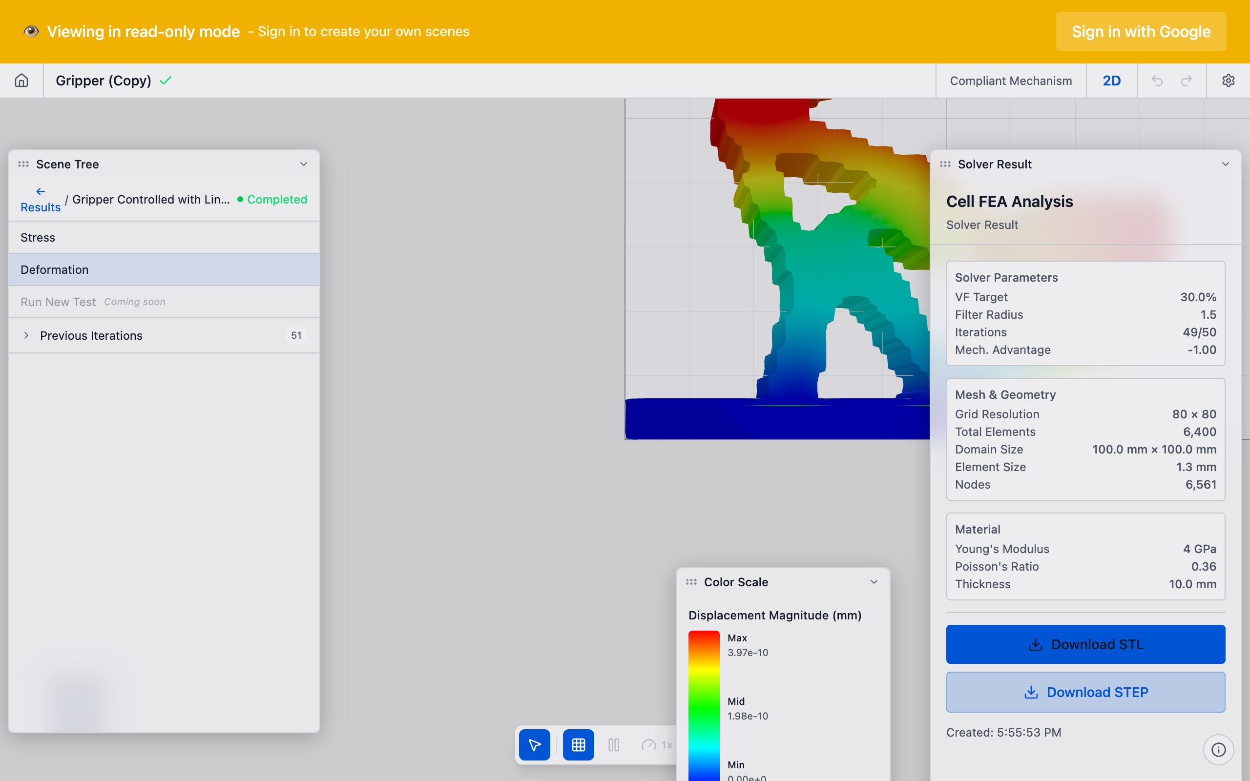
Color Mapping
deFlex visualizes the material layout using a color map. The default mapping shows:
- Void regions as the background (empty space)
- Solid regions in a solid color (the mechanism structure)
- Intermediate regions in lighter shades (transition zones)
The threshold slider in the results viewer lets you adjust the cutoff between "solid" and "void" for visualization purposes. Setting the threshold to 0.5 means elements with density > 0.5 appear solid, and elements below appear void.
Experiment with the threshold slider to understand the density distribution. If the design looks substantially different at thresholds of 0.3 versus 0.7, there are significant gray regions — the design may benefit from more iterations or adjusted parameters. If the design looks the same across a wide threshold range (0.3 to 0.7), the material layout is crisp and well-converged.
Evaluating Results
Signs of a Good Result
A high-quality optimized topology has these characteristics:
Clear, connected load paths: material forms continuous structural members connecting the input preserve to the output preserve through the fixed preserves. You can visually trace the path that force follows through the mechanism.
Crisp solid/void boundaries: most elements are near 0 or 1, with narrow transition zones. Extensive gray regions indicate the solver has not fully converged or the problem is ill-conditioned.
Meaningful flexure regions: thin sections of material where the mechanism bends. These are the "joints" of the compliant mechanism. They should appear at logical locations between structural members.
Symmetric design (when expected): if the problem has geometric symmetry (symmetric design space, symmetric preserve placement), the result should be approximately symmetric. Significant asymmetry suggests the solver converged to a local minimum.
Preserve connectivity: all preserves (input, output, fixed) should be connected to the mechanism structure. An isolated preserve means the optimizer could not find a viable load path to it.
Signs of a Problem
Disconnected material islands: floating blobs of material not connected to any preserve. These are structurally useless and indicate a problem with the solver setup. Possible causes: volume fraction too low, design space too large, or competing constraints.
All material concentrated at one preserve: the solver is solving a trivial problem — all the load path work happens in one small region. Usually caused by preserves being too close together or a degenerate pair configuration.
Uniform gray field: the solver did not converge. Densities are still near the initial value (the volume fraction). Increase the iteration limit or check for setup errors.
Thin tendrils or single-element connections: the mesh resolution is too coarse for the features the solver wants to create. Increase resolution or increase volume fraction.
A "bad-looking" result almost always indicates a problem with the setup, not the solver. The solver faithfully solves the problem you defined. If the result is not what you expected, revisit your preserve placement, directions, pairs, volume fraction, and design space.
What to Look For
Load Path Analysis
Trace the force path through the mechanism:
- Start at the input preserve — force enters here
- Follow the solid material — structural members carry force through the design space
- Identify flexure points — thin regions where the mechanism bends
- Arrive at the output preserve — displacement occurs here
- Continue to fixed preserves — reaction forces are absorbed here
A good mechanism has a clear, logical load path. If you cannot trace a continuous path from input through output to fixed preserves, the result is likely degenerate.
Flexure Identification
Flexures are the functional elements of the compliant mechanism — the thin regions that allow controlled bending. In the material layout, they appear as:
- Narrow connections (2-4 elements wide) between bulkier structural members
- Regions of slightly reduced density (0.7-0.9) adjacent to fully solid regions
- Necked-down sections at member junctions
The number, position, and orientation of flexures determine the mechanism's behavior:
- Few flexures, centrally located: simple, robust mechanism (like a lever with a single hinge)
- Many flexures, distributed: complex mechanism with multiple degrees of compliance
- Flexures near preserves: mechanism bends close to the attachment points
- Flexures far from preserves: mechanism bends in the interior, preserves are on rigid end-effectors
Output Displacement
The solver reports the output displacement — the displacement at the output preserve in the specified direction. This is the primary performance metric. Compare it to your requirements:
- Is the displacement sufficient for your application?
- How does it compare to the input displacement? (Ratio gives the mechanical advantage)
- Is the displacement consistent with the mechanism topology? (A very stiff-looking mechanism should not produce large output displacement)
Compliance Value
For structural stiffness problems (thermal flexure), the solver reports the final compliance value. Lower compliance means a stiffer structure. Check that:
- Compliance is finite and positive (0 < C < some reasonable upper bound)
- Compliance decreased monotonically through iterations (checked automatically by benchmarks)
- The final compliance is significantly lower than the initial (uniform density) compliance
Post-Processing
Thresholding for Manufacturing
The raw material layout contains continuous values. For manufacturing, you need a binary (solid/void) design. The simplest approach is thresholding:
- Set a density cutoff (typically 0.5)
- Elements above the cutoff become solid
- Elements below the cutoff become void
This produces a staircase boundary on the structured grid. Smoothing and contouring algorithms can extract a cleaner boundary.
The choice of threshold affects the manufactured part's volume and performance. A lower threshold (0.3) includes more material, making the part heavier but stiffer. A higher threshold (0.7) includes less material, producing a lighter but potentially weaker part. The "correct" threshold depends on your manufacturing process and performance requirements.
Extracting Key Metrics
From the converged result, extract these metrics for design evaluation:
| Metric | What It Tells You |
|---|---|
| Output displacement | Primary performance — does the mechanism move enough? |
| Compliance | Structural stiffness — is the mechanism rigid enough? |
| Volume fraction (actual) | Material usage — should match the specified constraint |
| Max intermediate density | Convergence quality — lower is better (ideally < 0.1) |
| Number of connected components | Topology quality — should be 1 (single connected part) |
Comparison Across Runs
When iterating on a design, compare results across runs:
- Keep preserve placement constant and vary volume fraction to see the trade-off
- Keep all parameters constant and vary mesh resolution to check mesh independence
- Vary K_p_max to explore the stiffness-flexibility trade-off
Document each run's parameters and results. The material layout visualization and convergence plot together tell the full story.
Troubleshooting
Result is a solid block: volume fraction is too high or K_p_max is extreme. Reduce volume fraction or lower K_p_max.
Result is empty (all void): the solver could not find a viable load path. Check preserve placement and pair configuration.
Result has many disconnected pieces: volume fraction is too low or the design space is too large relative to the preserve spacing. Increase volume fraction.
Result looks good but output displacement is near zero: the mechanism topology is stiff but does not transmit motion effectively. This can happen when K_p_max is too high. Lower K_p_max.
Result changes dramatically with small parameter changes: the problem is sensitive or near a bifurcation point. Multiple locally optimal solutions exist. This is not a bug — it reflects the nature of the problem.
See Also
- Design Optimization — the process that produces the material layout
- Convergence — determining when the result is ready
- Volume Fraction — the material budget that shapes the design
- Pairs — the stiffness coupling that affects mechanism behavior
- Compliant Mechanisms — understanding the mechanism the result represents